Lecture 03 - Local parametric optimization in MR control PDF

| Title | Lecture 03 - Local parametric optimization in MR control |
|---|---|
| Course | Adaptive Control Systems |
| Institution | Binghamton University |
| Pages | 20 |
| File Size | 1.9 MB |
| File Type | |
| Total Downloads | 110 |
| Total Views | 143 |
Summary
Local parametric optimization in MR control...
Description
ECE 517 LECTURE 03
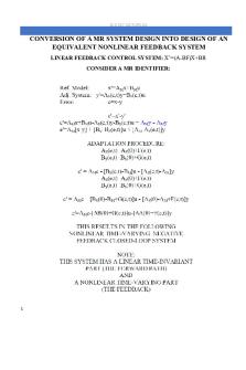
CONVERSION OF A MR SYSTEM DESIGN INTO DESIGN OF AN EQUIVALENT NONLINEAR FEEDBACK SYSTEM LINEAR FEEDBACK CONTROL SYSTEM: X’=(A-BF)X+BR CONSIDER A MR IDENTIFIER:
1
ECE 517 LECTURE 03
2
ECE 517 LECTURE 03
3
ECE 517 LECTURE 03
LOCAL PARAMETRIC OPTIMIZATION
GRADIENT MINIMIZATION:
4
ECE 517 LECTURE 03
5
ECE 517 LECTURE 03
6
ECE 517 LECTURE 03
7
ECE 517 LECTURE 03
8
ECE 517 LECTURE 03
9
ECE 517 LECTURE 03
10
ECE 517 LECTURE 03
SIMULATION STUDY OF A MR PARAMETER IDENTIFIER USING LOCAL PARAMETRIC OPTIMIZATION: Parallel configuration:
Adjustable system:
~ ~ ~ b2 s 2 b1 s b0 b2 s2 b1 s b0 ~ y( s) 3 x(s) and y (s ) 3 ~ 2 ~ ~ x (s ) s a2 s 2 a1s a0 s a2 s a1s a 0 e( s) y( s) ~y( s)
~ ~ ~ ~ ~ ~ b2 b2 (e,t ), b1 b1 ( e, t ), b0 b0 (e, t ) ~ ~ ~ a2 ~ a2 (e,t ), ~ a1 ~ a1( e, t ), a a0 (e, t ) 0 2 ~ 2 ~ ~ b2 s b1 s b0 ~ 2 Q( s, t ) e( s) [ y( s) y ( s)] y ( s) 3 ~ 2 ~ x (s ) s a2 s a1s ~ a0 2
11
ECE 517 LECTURE 03
12
ECE 517 LECTURE 03
~ db2 ~ ~ Q (s , t ) Q (s , t ) and b2( e, t) b2 (0) C2 C2 ~ dt ~ dt b2 b2 ~ ~ ~ db1 Q( s, t) Q( s, t) and b1 (e, t ) b1 (0) C1 C1 ~ ~ dt dt b1 b1 ~ ~ ~ Q( s, t) Q( s, t) db0 and b0( e, t) b0 (0) C0 C0 ~ ~ dt dt b0 b0 ~ da Q( s, t ) Q( s, t ) 2 and a~2 (e ,t ) a~2 (0) D2 D2 ~ dt ~ dt a2 a 2 ~ da1 Q( s, t ) Q( s, t ) a1( e, t) ~a1(0) D1 and ~ D1 ~ dt dt a a~1 1 ~ da0 Q ( s, t ) Q( s, t ) a0 (e,t ) a~0 (0) D0 and ~ D0 ~ dt ~ dt a a 0
13
0
ECE 517 LECTURE 03
14
ECE 517 LECTURE 03
Do not be surprised: although the gradient application results in the decrease of the criterion value, the parameter estimates do not converge to their “true” values. Successful parameter estimation requires that the input signal, driving the system, satisfy additional special requirements. Also, running the simulation for longer time may result in the divergence of the minimization procedure: the stability consideration cannot be incorporated in gradient minimization
15
ECE 517 LECTURE 03
16
ECE 517 LECTURE 03
17
ECE 517 LECTURE 03
18
ECE 517 LECTURE 03
EE 517 Homework Assignment #2 1. a) List factors that necessitate the use of adaptive control b) Give a descriptive example of a model reference control system that maintains the required performance despite varying operational conditions c) Give a descriptive example of a control system that maintains the required performance by utilizing the principle of feedforward control
2. Provide the description and matrix diagram of a model reference control system with signal adaptation and model reference state estimator that has a series-parallel configuration and parametric adaptation. Describe the operation of this system. Explain how the negative feedback principle is applied in this system.
3. Provide the description and matrix diagram of a model reference control system with parametric adaptation and model reference state estimator that has a parallel configuration and signal adaptation. Describe the operation of this system. Explain how the duality in model reference control works in this system.
4. A model reference system identifier/parameter estimator is utilized to obtain a mathematical model of a physical process in the form GS (s )
1 s 0 s 1s 0 2
Derive the adaptation mechanism utilizing the local parametric adaptation for the solution of this problem. Develop a simulation setup showing the operation of this system in the Simulink or Vissim environment and investigate the system operation
19
ECE 517 LECTURE 03
EE 517 Homework Assignment #3 A control system has to be designed for a first order controlled plant, transfer function G(s)
b , with poorly known parameters. s a
The design specifications call for the settling time of 1 sec and the overshoot of the system step response of approximately zero % Utilize local parametric optimization of the model reference approach to design a control system that would comply with the design specifications in spite of poorly known parameters of the controlled plant. a) Define and document the reference model. b) Establish the mathematical description and schematic of the entire adaptive control system c) Utilize the local parametric optimization approach (MIT rule) to develop an adaptation mechanism capable of adjusting parameters of the feedback controller and the input filter of the system. Provide all derivations d) Assume the transfer function of the “true plant” to be GTRUE (s)
.016 . s .029
Implement the adaptive control system using simulation software. e) Drive the system by a square wave-type reference signal with period of 3 sec. Choose the gains of the adaptation mechanism to demonstrate the gradual arrival of the system to the desired operation. Demonstrate the convergence of the system error and adjustable parameters of the controller. f) Provide the plot of the control effort. Note that in real life, the feasibility of adaptive control is limited by the allowable magnitude of the control effort. To test this reality, register the maximum magnitude of the control effort, then limit the magnitude of the control effort to 80% and 60% of the maximum value and repeat simulation runs. Document the results.
20...
Similar Free PDFs

Local government in India
- 18 Pages

Parametric vs Nonparametric Stats
- 18 Pages

Non Parametric Var
- 3 Pages

Non - parametric Friedman test
- 38 Pages

Ldr optimization
- 3 Pages

EE273 - lecture 03-long
- 30 Pages

Mr Know it all - Lecture Notes
- 5 Pages

CA M 03 Control System Toolbox
- 19 Pages
Popular Institutions
- Tinajero National High School - Annex
- Politeknik Caltex Riau
- Yokohama City University
- SGT University
- University of Al-Qadisiyah
- Divine Word College of Vigan
- Techniek College Rotterdam
- Universidade de Santiago
- Universiti Teknologi MARA Cawangan Johor Kampus Pasir Gudang
- Poltekkes Kemenkes Yogyakarta
- Baguio City National High School
- Colegio san marcos
- preparatoria uno
- Centro de Bachillerato Tecnológico Industrial y de Servicios No. 107
- Dalian Maritime University
- Quang Trung Secondary School
- Colegio Tecnológico en Informática
- Corporación Regional de Educación Superior
- Grupo CEDVA
- Dar Al Uloom University
- Centro de Estudios Preuniversitarios de la Universidad Nacional de Ingeniería
- 上智大学
- Aakash International School, Nuna Majara
- San Felipe Neri Catholic School
- Kang Chiao International School - New Taipei City
- Misamis Occidental National High School
- Institución Educativa Escuela Normal Juan Ladrilleros
- Kolehiyo ng Pantukan
- Batanes State College
- Instituto Continental
- Sekolah Menengah Kejuruan Kesehatan Kaltara (Tarakan)
- Colegio de La Inmaculada Concepcion - Cebu


