R Cheat Data - R CHEET SHEETS PDF

| Title | R Cheat Data - R CHEET SHEETS |
|---|---|
| Author | Wanyun Huang |
| Course | Statistics |
| Institution | Katholieke Universiteit Leuven |
| Pages | 4 |
| File Size | 169.3 KB |
| File Type | |
| Total Downloads | 101 |
| Total Views | 149 |
Summary
R CHEET SHEETS...
Description
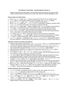
The Ultimate R Cheat Sheet – Data Management (Version 4) Google “R Cheat Sheet” for alternatives. The best cheat sheets are those that you make yourself! Arbitrary variable and table names that are not part of the R function itself are highlighted in bold. Import, export, and quick checks
dat1=read.csv("name.csv") to import a standard CSV file (first row are variable names). attach(dat1) to set a table as default to look for variables. Use detach() to release. dat1=read.delim("name.txt") to import a standard tab-delimited file. dat1=read.fwf("name.prn", widths=c(8,8,8)) fixed width (3 variables, 8 characters wide). ?read.table to find out more options for importing non-standard data files. dat1=read.dbf("name.dbf") requires installation of the foreign package to import DBF files. head(dat1) to check the first few rows and variable names of the data table you imported. names(dat1) to list variable names in quotation marks (handy for copy and paste to code). data.frame(names(dat1)) gives you a list of your variables with the column number indicated, which can be handy for sub-setting a data table (see next page) nrow(dat1) and ncol(dat1) returns the number of rows and columns of a data table. length(dat1$VAR1[!is.na(dat1$VAR1)] returns a count of non-missing values in a variable. str(dat1) to check variable types, which is useful to see if the import executed correctly. write.csv(results, "myresults.csv", na="", row.names=F) to export data. Without the option statements, missing values will be represented by NA and row numbers will be written out.
Data types and basic data table manipulations
There are three important variable types: numeric, character and factor (a double variable with a numeric and character value). You can query or assign types: is.factor() or as.factor(). If you import a data table, variables that contain one or more character entries will be set to factor. You can force them to numeric with this: as.numeric(as.character(dat1$VAR1)) After subsetting or modification, you might want to refresh factor levels with droplevels(dat1) Data tables can be set as.data.frame(), as.matrix(), as.distance() names(dat1)=c("ID", "X", "Y", "Z") renames variables. Note that the length of the vector must match the number of variable you have (four in this case). row.names(dat1)=dat1$ID. assigns an ID field to row names. Note that the default row names are consecutive numbers. In order for this to work, each value in the ID field must be unique. To generate unique and descriptive row names that may serve as IDs, you can combine two or more variables: row.names(dat1)=paste(dat1$SITE, dat1$PLOT, sep="-") If you only have numerical values in your data table, you can transpose it (switch rows and columns): dat1_t=t(dat1). Row names become variables, so run the row.names() function above first. dat1[order(X),] orders rows by variable X. dat[order(X,Y),] orders rows by variable X, then variable Y. dat1[order(X,-Y),]. Orders rows by variable X, then descending by variable Y. fix(dat1) to open the entire data table as a spreadsheet and edit cells with a double-click.
Creating systematic data and data tables
c(1:10) is a generic concatenate function to create a vector, here numbers from 1 to 10. seq(0, 100, 10) generates a sequence from 0 to 100 in steps of 10. rep(5,10) replicates 5, 10 times. rep(c(1,2,3),2) gives 1 2 3 1 2 3. rep(c(1,2,3), each=2) gives 1 1 2 2 3 3. This can be useful to create data entry sheets for experimental designs. data.frame(VAR1=c(1:10), VAR2=seq(10, 100, 10), VAR3=rep( c("this", "that"),5)) creates a data frame from a number of vectors. expand.grid(SITE=c("A","B"),TREAT=c("low","med","high"), REP=c(1:5)) is an elegant method to create systematic data tables.
Creating random data and random sampling
rnorm(10) takes 10 random samples from a normal distribution with a mean of zero and a standard deviation of 1 runif(10) takes 10 random samples from a uniform distribution between zero and one. round(rnorm(10)*3+15)) takes 10 random samples from a normal distribution with a mean of 15 and a standard deviation of 3, and with decimals removed by the rounding function. round(runif(10)*5+15) returns random integers between 15 and 20, uniformly distributed. sample(c("A","B","C"), 10, replace=TRUE) returns a random sample from any custom vector or variable with replacement. sample1=dat1[sample(1:nrow(dat1), 50, replace=FALSE),] takes 50 random rows from dat1 (without duplicate sampling). This can be handy for bootstrapping or to run quick test analyses on subsets of very large datasets.
Sub-setting data tables, conditional subsets
dat1[1:10, 1:5] returns the first 10 rows and the first 5 columns of table dat1. dat2=dat1[50:70,] returns a subset of rows 50 to 70. cleandata=dat1[-c(2,7,15),] removes rows 2, 7 and 15. selectvars=dat1[,c("ID","YIELD")] sub-sets the variables ID and YIELD selectrows=dat1[dat1$VAR1=="Site 1",] sub-sets entries that were measured at Site 1. Possible conditional operators are == equal, != non-equal, > larger, < smaller, >= larger or equal,...
Similar Free PDFs

R Cheat Data - R CHEET SHEETS
- 4 Pages

R Cheat sheet R-Markdownpdf
- 2 Pages

R Markdown Cheat Sheet
- 2 Pages

R-Cheat-Sheet
- 4 Pages

cheat sheet programmation R
- 2 Pages

R cheat sheet 3
- 2 Pages

Base r cheat sheet
- 2 Pages

R-cheatsheet data-wrangling
- 2 Pages

R For Data Science
- 520 Pages

Gage R&R ejemplo - G R&R
- 23 Pages

R
- 1 Pages

Data.table en r cheat sheet
- 1 Pages

Cheat sheat med R hjælp
- 21 Pages

R Cheat sheet 1 - non
- 2 Pages
Popular Institutions
- Tinajero National High School - Annex
- Politeknik Caltex Riau
- Yokohama City University
- SGT University
- University of Al-Qadisiyah
- Divine Word College of Vigan
- Techniek College Rotterdam
- Universidade de Santiago
- Universiti Teknologi MARA Cawangan Johor Kampus Pasir Gudang
- Poltekkes Kemenkes Yogyakarta
- Baguio City National High School
- Colegio san marcos
- preparatoria uno
- Centro de Bachillerato Tecnológico Industrial y de Servicios No. 107
- Dalian Maritime University
- Quang Trung Secondary School
- Colegio Tecnológico en Informática
- Corporación Regional de Educación Superior
- Grupo CEDVA
- Dar Al Uloom University
- Centro de Estudios Preuniversitarios de la Universidad Nacional de Ingeniería
- 上智大学
- Aakash International School, Nuna Majara
- San Felipe Neri Catholic School
- Kang Chiao International School - New Taipei City
- Misamis Occidental National High School
- Institución Educativa Escuela Normal Juan Ladrilleros
- Kolehiyo ng Pantukan
- Batanes State College
- Instituto Continental
- Sekolah Menengah Kejuruan Kesehatan Kaltara (Tarakan)
- Colegio de La Inmaculada Concepcion - Cebu

