Econ2020a 18 ps01 1 PDF

| Title | Econ2020a 18 ps01 1 |
|---|---|
| Author | Patricia Walters |
| Course | Microeconomic Theory I |
| Institution | Harvard University |
| Pages | 3 |
| File Size | 110.2 KB |
| File Type | |
| Total Downloads | 119 |
| Total Views | 137 |
Summary
Consumer theory assignment...
Description
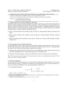
API 111 / ECON 2020a / HBS 4010 (Fall 2018) Maciej H. Kotowski / Harvard University
Problem Set 1 Due: September 17, 2018 at 12.00
• Legibly write your name (and the names of any collaborators) on your independently written-up solutions. • Submit your solutions to the assignment drop box. Do not bring solutions to lecture. • Show your work. Include brief and precise explanations of intuition and derivations as appropriate. • Help us out.
Enclose final answers with a box.
1. College Admissions and the Stability of Marriage This question lets you practice applying the deferred acceptance algorithm proposed by David Gale and Lloyd Shapley (“College Admissions and the Stability of Marriage,” American Mathematical Monthly 69(1):9–15, 1962). On page 13, the authors write that a “reader may amuse himself” by applying the deferred acceptance algorithm to find a stable matching in the example provided in the paper. In their example, men are labeled with Greek letters; women are labeled with Roman letters. a) Find a stable matching in the example on page 13 using the “man-proposing” deferred acceptance algorithm. b) Find a stable matching in the example on page 13 using the “woman-proposing” deferred acceptance algorithm. c) Find all remaining stable matchings in this economy. (If there are no other stable matchings, carefully explain why.)
2. Constructing Unusual Utility Functions In some applications we may wish to assume a decision maker exhibits an unusual habit or quirk. In each of the following cases propose a utility function that models the described behavior. Be sure to carefully define the choice set over which the decision maker’s preferences are defined. a) Someone who would rather be the richest man in a poor neighborhood rather than the poorest man in the richest neighborhood (even if that means being poorer in absolute terms). b) Someone who prefers mangoes to apples, but will refuse to take the last mango from a fruit basket.1 Hint: There are many correct answers to this question and its easy to overcomplicate your answer. Try to keep your model as simple as possible. 3. Preference Relations Let x, y ∈ R2+ denote two consumption vectors and consider the following preferences defined over two goods. Do the preferences satisfy (i) continuity, (ii) transitivity, (iii) monotonicity, and (iv) local non-satiation? In each case, sketch the “indifference curve” passing through the bundle (2, 2).2 a) Lexicographic Preferences: x ≻ y ⇐⇒ and x ∼ y if x1 = y1 and x2 = y2 .
x1 > y1 or (x1 = y1 and x2 > y2 )
1 This case is a simplification of an example due to Amartya Sen. See Amartya Sen, “Maximization and the Act of Choice,” Econometrica 65 no. 4 (1997):745–779. 2 Formally, you should indicate the set {(x1 , x2 ) ∈ R2+ : (x1 , x2 ) ∼ (2, 2)}.
1
b) If (x1 + x2 − y1 − y2 ) > 1, then x ≻ y. If |x1 + x2 − y1 − y2 | ≤ 1, then x ∼ y.
4. Convex Preferences and Quasi-Concave Utility Functions L Let % be a binary relation defined on R+ that is complete and transitive. Let x, y ∈ RL+ be consumption vectors. Here are some important definitions: • The relation % is convex if for all x and y such that x % y, αx + (1 − α)y % y for all α ∈ [0, 1].3 L • The function u: R+ → R is concave if for all x, y ∈ RL+ , and α ∈ [0, 1], u(αx + (1 − α)y) ≥ αu(x) + (1 − α)u(y). L • The function u: RL + → R is quasi-concave if for all x, y ∈ R + , and α ∈ [0, 1], u(αx + (1 − α)y) ≥ min{u(x), u(y)}.
a) Read section 3.2 of the Miller notes. You can find them online: b) Suppose the utility function u(·) represents the convex preference relation %. Show that u(·) is a quasiconcave function. c) Suppose a quasi-concave utility function u(·) represents a preferences relation %. Show that % is a convex preference relation. d) Suppose u(·) is a concave function. Show that u(·) is quasi-concave. e) Suppose there is only one good, i.e. L = 1. Consider the utility function u(x) = x21 . Verify that this function is not concave. Verify that it is quasi-concave. f) Suppose there are two goods, i.e. L = 2. Consider the utility function u(x) = x21 x22 . Verify that this function is not concave. Verify that it is quasi-concave. g) Give an example of preferences that are monotone and continuous but not convex. State a practical situation where non-convex preferences seem reasonable.
5. Canonical Utility Functions and Walrasian Demand Suppose there are two goods, 1 and 2. For each of the following utility functions, find the Walrasian demand correspondence for each good.4 Let pℓ > 0 be the price of good ℓ and let w > 0 the consumer’s wealth. (You may wish to draw pictures of indifference curves and budget sets to help you.) a) Cobb-Douglas: u(x1 , x2 ) = xα1 x2β for α, β > 0. b) Logarithmic Quasi-linear: u(x1 , x2 ) = α log(x1 ) + x2 , α > 0. Remark: In this course, “log(·)” always stands for the natural logarithm, i.e. log(e) = 1. On your calculator, the natural logarithm might be denoted by “ln(·).” c) Linear: u(x1 , x2 ) = αx1 + βx2 for α, β > 0. d) Generalized Leontief: u(x1 , x2 ) = min{αx1 , βx2 } for α, β > 0. Keep your answers to this question handy—it will save you work in the future. 3 4
By writing “αx + (1 − α)y” we mean a bundle where the quantity of each good ℓ is αxℓ + (1 − α)yℓ . We use the term correspondence since there may be prices at which the consumer is indifferent among many bundles.
2
6. Utility Maximization with a Quantity Discount Suppose Betty has wealth w = 32 and she consumes two goods, rice (x1 ) and vegetables (x2 ). The regular prices of these goods per kilogram are p1 = 4 and p2 = 4 respectively. Betty’s utility function is u(x1 , x2 ) = x1 x2 . Suppose that when Betty buys more than x ˜1 kilograms of rice, she qualifies for a price discount. Specifically, rather than paying 4 dollars per kilogram, Betty pays only p˜1 = 1 per kilogram in excess of x ˜1 . For example, if x ˜1 = 4 and Betty buys 10 kilograms of rice, she pays 4 × $4 + (10 − 4) × $1 = $16 + $6 = $22. (She pays $4/kg on the first x ˜1 kilograms and $1/kg on any remainder.) a) Suppose x ˜1 = 6. Find Betty’s utility-maximizing bundle. b) Suppose x ˜ 1 = 5. Find Betty’s utility-maximizing bundle. c) Suppose x ˜ 1 = 16/3. Find Betty’s utility-maximizing bundle(s). d) Provide some intuition for the results in parts (a)–(c).
Additional Practice Problems (Do Not Hand In) 7. Pedantically Proving Transitivity (Jehle & Reny 1.4) Let % be a complete and transitive preference relation defined on the set X. Using %, we can define two new relations on X : a) The relation ≻ is defined as “x ≻ y if and only if x % y and y 6% x.” b) The relation ∼ is defined as “x ∼ y if and only if x % y and y % x.” Using the definitions, carefully argue that ≻ and ∼ are transitive relations. Are they complete? 8. “Separable” Utility Functions [Rubinstein 2012, Problem 4.6] For tractability, many studies assume consumers have “separable” preferences. This question explores some properties of preferences meeting this criterion. We say that a preference relation % satisfies separability if PL it can be represented by an additive utility function. For example, the function u(x) = ℓ=1 vℓ (xℓ ) for any x = (x1 , . . . , xL ) is additively separable. a) Suppose a consumer has Cobb-Douglas preferences over a set of goods which are available only in strictly positive quantities. Are his preferences separable? b) Show that separable preferences satisfy the following condition: (⋆) For any subset of commodities J , and for any bundles a, b, c, d, we have: (aJ , c−J ) % (bJ , c−J ) ⇐⇒ (aJ , d −J ) % (bJ , d −J ) where (xJ , y−J ) is the vector that takes the components of x for any k ∈ J and takes the components of y for any k ∈ / J .5 c) Show that for the case of two goods (K = 2), separable preferences satisfy the “Hexagon-condition”: If (a, b) % (c, d) and (c, e) % (f, b), then (a, e) % (f, d ). d) Give an example of a continuous preference relation that satisfies condition (⋆), defined above, and does not satisfy separability. (Hint: Consider only two goods and draw a picture with indifference curves.) 5
For example, if K = 5 and J = {1, 2, 5}. Then, (xJ , y−J ) = (x1 , x2 , y3 , y4 , x5 ).
3...
Similar Free PDFs

Econ2020a 18 ps01 1
- 3 Pages

Semana 18 2013 - 1 - Apuntes 18
- 98 Pages

John 1:6-18
- Pages

Chapter 18 - Lecture 1
- 37 Pages

ANAT057-18 1 0
- 14 Pages

Temario - Apuntes 1-18
- 107 Pages

Chap 1-18 - Stuff
- 42 Pages

Lösung 1 - WS17/18
- 5 Pages

18 - lab 18
- 4 Pages

18 - Lecture notes 18
- 5 Pages

TEMA 18 - Apuntes 18
- 3 Pages

Sepsis lecture 1 2017 18
- 9 Pages

Cultural Autobiography 1-21-18
- 2 Pages

BUSN3008 S 1 18 - Summary
- 12 Pages

Samenvatting Chinees 1 LES 18
- 1 Pages
Popular Institutions
- Tinajero National High School - Annex
- Politeknik Caltex Riau
- Yokohama City University
- SGT University
- University of Al-Qadisiyah
- Divine Word College of Vigan
- Techniek College Rotterdam
- Universidade de Santiago
- Universiti Teknologi MARA Cawangan Johor Kampus Pasir Gudang
- Poltekkes Kemenkes Yogyakarta
- Baguio City National High School
- Colegio san marcos
- preparatoria uno
- Centro de Bachillerato Tecnológico Industrial y de Servicios No. 107
- Dalian Maritime University
- Quang Trung Secondary School
- Colegio Tecnológico en Informática
- Corporación Regional de Educación Superior
- Grupo CEDVA
- Dar Al Uloom University
- Centro de Estudios Preuniversitarios de la Universidad Nacional de Ingeniería
- 上智大学
- Aakash International School, Nuna Majara
- San Felipe Neri Catholic School
- Kang Chiao International School - New Taipei City
- Misamis Occidental National High School
- Institución Educativa Escuela Normal Juan Ladrilleros
- Kolehiyo ng Pantukan
- Batanes State College
- Instituto Continental
- Sekolah Menengah Kejuruan Kesehatan Kaltara (Tarakan)
- Colegio de La Inmaculada Concepcion - Cebu
