Extrapolation Formula in mathematics PDF

| Title | Extrapolation Formula in mathematics |
|---|---|
| Author | wafula moses |
| Course | information technology |
| Institution | College MCS |
| Pages | 17 |
| File Size | 781 KB |
| File Type | |
| Total Downloads | 20 |
| Total Views | 135 |
Summary
he exciton energy levels move "down" from the free exciton level by an amount equal to the binding energy of the electron to the isoelectronic dopant...
Description
Extrapolation Formula Let us consider the two endpoints in a linear graph (x1, y1) and (x2, y2) where the value of the point “x” is to be extrapolated, and then the extrapolation formula is given as
y(x)=y1+x−x1x2−x1(y2−y1)
Extrapolation Graph As we know, extrapolation is a process of predicting the data point about the outside of a curve when a few points are given. In the example given below, the known data are x1, x2, x3. Finding the point x4 is known as extrapolation point.
Extrapolation Example Question: The two given points that lie on the straight line is (1, 5) and (4, 10). Determine the value of y at x = 5 on the straight line using a linear extrapolation method. Solution: Given: x1 = 1 ,y1 = 5
and x2 = 4, y2 = 10 The linear extrapolation formula is given as;
y(x)=y1+x−x1x2−x1(y2−y1) Substitute the known values in the given formula, y(5) = 5 +[(5-1)/(4-1)](10-5) y(5) = 5 + (4/3) (5) y(5) = 5 + 6.67 y(5)= 11.67 Therefore y(5) = 11.67
Finite difference table A finite difference is a mathematical expression of the form f (x + b) − f (x + a). If a finite difference is divided by b − a, one gets a difference quotient. The approximation of derivatives by finite differences plays a central role in finite difference methods for the numerical solution of differential equations, especially boundary value problems. FINITE DIFFERENCES When you learned about ordinary differential equations with constant coefficients, an operator D=d/dx was introduced. A corresponding approach may be adopted in the case of finite differences. Of course, you know that differentiation is arrived at by a limiting process applied to differences:
The calculus of finite differences deals with the right hand side of this equation without the limit. One common use of finite differences, known to you, was in linear interpolation. Using tables at school, for example of logarithms or trigonometric
functions, you interpolated linearly. The tables were designed so that your result would never be out by more than 0.5 of the last digit. EXAMPLE log 10x
In order to interpolate log 2.036 you wrote
Today, your calculator gives .3087778 = .3088. The shorthand for such a table is
DIFFERENCE TABLES While it is not essential, we will concentrate on uniform difference tables, i.e., when the values of functions are given at regular intervals. Also, it is customary to omit decimal points and forward zeroes, so that the earlier table for logarithms would become
We see that tables can be rough (involve large intervals) when a function changes slowly, and become fine when it changes fast. The first table above shows that the first differences are almost the same. They oscillate between 22 and 21, whence the second difference oscillates in sign. This is the result of round off, an error from the function's point of view. Finite difference tables can be used to discover errors in tabulated functions. One speaks of noise level which in the first difference can only be 1, since the entries are rounded-off, i.e., the last digit may be incorrect by0.5.
However, such errors build up quickly:
This phenomenon indicates the presence of noise due to An estimate of expected noise level is given by the table:
round-off in data.
Like throughout mathematics, notation tends to make life easier, although at first it may appear to be a hurdle. SHIFT OPERATOR In the difference table for ln x, the first column corresponded to equi-distant data values of f(x):
The shift operator E is defined by the relation
where k need not be positive or an integer:
Why should we be concerned with fractional powers of E? We might use this formula to start with only every second value in a table, and later switch over to every value. FORWARD BACKWARD AND CENTRAL DIFFERENCES In the difference table above, we formed the first differences fj+1-fj , which are now given in terms of the shift operator E by
since
Similarly,
In this manner, binomial coefficients enter into the finite difference calculus, since
The central difference operator is defined by:
and the backward operator by:
The corresponding Differences Tables are
The values of the forward and backward differences are the same, but they occupy different positions in the tables. The odd order central differences have other values, the even order differences agree with those of the other differences. This aspect of finite differences becomes important for interpolation. In order to interpolate function values at the beginning of a table, forward differences must used, because they have the largest number of differences at the centre of their table; central differences are used inside the table, and backward differences near the end. This becomes obvious when one rewrites tables so that the differences of different orders
with the same subscripts are written on one line. Then the front of the forward difference table slants backwards, that of the backward table forward, while the central difference table has triangular form:
Example 5.1 Construct a forward difference table for the following data
Solution: The Forward difference table is given below
Example 5.2 Construct a forward difference table for y = f(x) = x 3 + 2x + 1 for x = 1,2,3,4,5 Solution: y = f(x) = x3 + 2 x + 1 for x =1,2,3,4,5
Example 5.3 By constructing a difference table and using the second order differences as constant, find the sixth term of the series 8,12,19,29,42… Solution: Let k be the sixth term of the series in the difference table First we find the forward differences.
Given that the second differences are constant ∴ k – 55 = 3 k = 58 ∴ the sixth term of the series is 58
Example 5.4 Find (i) ∆eax (ii) ∆2ex (iii) ∆logx Solution:
Example 5.5
Evaluate Solution:
by taking ‘1’ as the interval of differencing.
Example 5.5
Evaluate
by taking ‘1’ as the interval of differencing.
Solution:
Example 5.7 Prove that f(4) = f(3) + Δf(2) + Δ2f(1) + Δ3f(1) taking ‘1’ as the interval of differencing. Solution:
We know that f(4) - f(3) = Δ f(4) f(4) - f(3) = Δ f(3) = Δ [ f(2) + Δf(2) ]
i.e.[ f(3) - f(2) = Δf(2) ]
= Δ f(2) + Δ2f(2) = Δ f(2) + Δ2[f(1)+ Δf(1)] f(4) = f(3) + Δf(2) + Δ2 f(1) + Δ3 f(1)
Example 5.8 Given U0 =1, U1 =11, U2 =21, U3 =28 and U4 =29 find Δ4U0 Solution: Δ4U0 = (E-1) 4U0
Tags :...
Similar Free PDFs

Extrapolation Formula in mathematics
- 17 Pages

IAL Mathematics Formula Book
- 32 Pages

Mathematics in Chemistry
- 6 Pages

Mathematics in the Modern World
- 12 Pages

LESSON PLAN IN MATHEMATICS 8
- 3 Pages

Graduate Texts in Mathematics 242
- 684 Pages
Popular Institutions
- Tinajero National High School - Annex
- Politeknik Caltex Riau
- Yokohama City University
- SGT University
- University of Al-Qadisiyah
- Divine Word College of Vigan
- Techniek College Rotterdam
- Universidade de Santiago
- Universiti Teknologi MARA Cawangan Johor Kampus Pasir Gudang
- Poltekkes Kemenkes Yogyakarta
- Baguio City National High School
- Colegio san marcos
- preparatoria uno
- Centro de Bachillerato Tecnológico Industrial y de Servicios No. 107
- Dalian Maritime University
- Quang Trung Secondary School
- Colegio Tecnológico en Informática
- Corporación Regional de Educación Superior
- Grupo CEDVA
- Dar Al Uloom University
- Centro de Estudios Preuniversitarios de la Universidad Nacional de Ingeniería
- 上智大学
- Aakash International School, Nuna Majara
- San Felipe Neri Catholic School
- Kang Chiao International School - New Taipei City
- Misamis Occidental National High School
- Institución Educativa Escuela Normal Juan Ladrilleros
- Kolehiyo ng Pantukan
- Batanes State College
- Instituto Continental
- Sekolah Menengah Kejuruan Kesehatan Kaltara (Tarakan)
- Colegio de La Inmaculada Concepcion - Cebu


