1010 WKW12 - USYD PDF

| Title | 1010 WKW12 - USYD |
|---|---|
| Author | Junlan Yang |
| Course | Introduction to Economic Statistics |
| Institution | University of Sydney |
| Pages | 4 |
| File Size | 179.1 KB |
| File Type | |
| Total Downloads | 12 |
| Total Views | 150 |
Summary
USYD...
Description
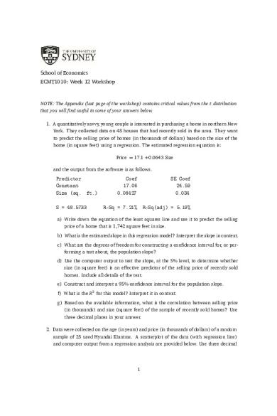
School of Economics ECMT1010: Week 12 Workshop
NOTE: The Appendix (last page of the workshop) contains critical values from the t distribution that you will find useful in some of your answers below. 1. A quantitatively savvy, young couple is interested in purchasing a home in northern New York. They collected data on 48 houses that had recently sold in the area. They want to predict the selling price of homes (in thousands of dollars) based on the size of the home (in square feet) using a regression. The estimated regression equation is: Price = 17.1 + 0.0643 Size and the output from the software is as follows.
Predictor Constant Size (sq. ft.) S = 48.5733
Coef 17.06 0.06427
SE Coef 24.59 0.034
R-Sq = 7.21%
R-Sq(adj) = 5.19%
a) Write down the equation of the least squares line and use it to predict the selling price of a home that is 1,742 square feet in size. b) What is the estimated slope in this regression model? Interpret the slope in context. c) What are the degrees of freedom for constructing a confidence interval for, or performing a test about, the population slope? d) Use the computer output to test the slope, at the 5% level, to determine whether size (in square feet) is an effective predictor of the selling price of recently sold homes. Include all details of the test. e) Construct and interpret a 95% confidence interval for the population slope. f) What is the R2 for this model? Interpret it in context. g) Based on the available information, what is the correlation between selling price (in thousands) and size (square feet) of the sample of recently sold homes? Use three decimal places in your answer. 2. Data were collected on the age (in years) and price (in thousands of dollars) of a random sample of 25 used Hyundai Elantras. A scatterplot of the data (with regression line) and computer output from a regression analysis are provided below. Use three decimal
1
places when reporting the results from any calculations, unless otherwise specified. The estimated regression equation is: Price = 15.3 − 1.71 Age
Predictor Constant Age S = 1.37179
Coef 15.2912 -1.7126
SE Coef 0.5840 0.1264
R-Sq = 88.9%
R-Sq(adj) = 88.4%
a) Use the scatterplot to determine whether we should have any major concerns about the conditions being met for using a linear model with these data. Explain briefly. b) What is the estimated slope in this regression model? Interpret the slope in context. c) Write down the equation of the least squares line and use it to predict the price of a used Hyundai Elantra that is 6 years old. d) What are the degrees of freedom for constructing a confidence interval for, or performing a test about, the population slope? e) Use the computer output to test the slope to determine whether age is an effective predictor of price. Use α = 0.05. Include all details of the test. f) Construct and interpret a 90% confidence interval for the population slope. g) What is the R2 for this model? Interpret it in context. h) Based on the available information, what is the correlation between age and price (in thousands of dollars) of used Hyundai Elantras? 3. In recent years, fast food restaurants have been required to publish nutrition information about the foods they serve. Nutrition information about a random sample of 15 McDonald’s lunch/dinner menu items (excluding sides and drinks) was obtained from their website. We wish to use the total fat content (in grams) to better understand the number of calories in the menu items at McDonald’s. Computer output from a regression analysis and a scatterplot (with regression line) of the data are provided below. Use
2
two decimal places when reporting the results from any calculations, unless otherwise specified. The estimated regression equation is: Calories = 137.1 + 15.06 Total Fat (g)
Predictor Constant Total Fat (g) S = 62.7442
Coef 137.08 15.055
SE Coef 40.64 5.149
R-Sq = 86.5%
R-Sq(adj) = 85.5%
a) Use the scatterplot to determine whether we should have any major concerns about the conditions being met for using a linear model with these data. Explain briefly. b) Write down the equation of the least squares line and use it to predict the number of calories in a menu item with 20 grams of fat. c) What is the estimated slope in this regression model? Interpret the slope in context. d) What are the degrees of freedom for constructing a confidence interval for, or performing a test about, the population slope? e) Use the computer output and α = 0.01 to test the slope to determine whether higher total fat content (g) predicts more calories. Include all details of the test. f) Construct and interpret a 99% confidence interval for the population slope. g) What is the R2 for this model? Interpret it in context. h) Based on the available information, what is the correlation between total fat content (g) and number of calories for McDonald’s lunch/dinner menu items in this sample?
3
Appendix Selected critical values from the t distribution by degrees of freedom (df ) Right tail probability df
0.05
0.025
0.01
0.005
8
1.860
2.306
2.896
3.355
9
1.833
2.262
2.821
3.250
13
1.771
2.160
2.650
3.012
23
1.714
2.069
2.500
2.807
24
1.711
2.064
2.492
2.797
46
1.679
2.013
2.410
2.687
49
1.677
2.010
2.405
2.680
67
1.668
1.996
2.383
2.651
98
1.661
1.984
2.365
2.627
4...
Similar Free PDFs

1010 WKW12 - USYD
- 4 Pages

Evidence - Summary - USYD LAWS5013
- 95 Pages

APA 6 Guide USYD
- 19 Pages

AG 1010
- 2 Pages

USYD Chemistry data sheet
- 4 Pages

Usyd academic calendar of2022
- 1 Pages

Draft User Guide USyd version
- 3 Pages

Family Law - Summary - USYD LAWS5132
- 104 Pages

COM 1010 Syllabus
- 12 Pages

English-1010-handbook
- 68 Pages

Assignment 1 - USyd Stock Exchange
- 13 Pages

Jv-1010 - Manual español
- 94 Pages

History 1010 lecture 12
- 6 Pages
Popular Institutions
- Tinajero National High School - Annex
- Politeknik Caltex Riau
- Yokohama City University
- SGT University
- University of Al-Qadisiyah
- Divine Word College of Vigan
- Techniek College Rotterdam
- Universidade de Santiago
- Universiti Teknologi MARA Cawangan Johor Kampus Pasir Gudang
- Poltekkes Kemenkes Yogyakarta
- Baguio City National High School
- Colegio san marcos
- preparatoria uno
- Centro de Bachillerato Tecnológico Industrial y de Servicios No. 107
- Dalian Maritime University
- Quang Trung Secondary School
- Colegio Tecnológico en Informática
- Corporación Regional de Educación Superior
- Grupo CEDVA
- Dar Al Uloom University
- Centro de Estudios Preuniversitarios de la Universidad Nacional de Ingeniería
- 上智大学
- Aakash International School, Nuna Majara
- San Felipe Neri Catholic School
- Kang Chiao International School - New Taipei City
- Misamis Occidental National High School
- Institución Educativa Escuela Normal Juan Ladrilleros
- Kolehiyo ng Pantukan
- Batanes State College
- Instituto Continental
- Sekolah Menengah Kejuruan Kesehatan Kaltara (Tarakan)
- Colegio de La Inmaculada Concepcion - Cebu


