Introductory Simulink Tutorial PDF

| Title | Introductory Simulink Tutorial |
|---|---|
| Course | Aerospace Systems, Modelling & Control |
| Institution | University of Hertfordshire |
| Pages | 3 |
| File Size | 226.8 KB |
| File Type | |
| Total Downloads | 101 |
| Total Views | 179 |
Summary
Introductory Simulink Tutorial...
Description
University of Hertfordshire School of Engineering & Technology
AN INTRODUCTORY TUTORIAL ON MATLAB/SIMULINK.
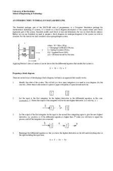
The Simulink package, part of the MATLAB suite of programmes, is a Computer Simulation package for mathematical modelling of systems. It is based on a block diagram description of the system where each block represents part of the system. Simulink models each block in turn and determines the way in which blocks interact. Before we can use Simulink we need to prepare a block diagram (or analogue diagram) of the system we wish to simulate. For this tutorial we shall simulate a mass/spring/damper system.
c
f
M
where M = Mass (1Kg), c = Damping Coefficient (3Ns/m), k = Spring Constant (2N/m), f(t) = Applied Force (10N) y(t) = Distance moved by the mass.
k y Applying Newton’s laws of motion it can be shown that the differential equation that models this system is:
y + 3y + 2y = f Preparing a block diagram There are several ways of developing a block diagram, but here is an approach that usually works. 1.
Identify the order of the system. This will tell you how many integrators you need in your diagram. (In this case two.) Draw these in the centre of a piece of paper with plenty of space around each one.
2.
Let the input to the first integrator be the highest derivative in the differential equation, in this case acceleration, y . Hence the output of this integrator will be the next highest derivative. (i.e. velocity, y )
3.
Let the output of the first integrator be the input to the second thus integrating again to give the next highest derivative. (i.e. position, y). If the differential equation is higher than 2nd order you will have to repeat this process until all the integrators are connected.
4.
Rearrange the differential equation so that you have the highest derivative on the left and everything else on the right including the input term.
y = f − 2y − 3y
5.
By placing a summer junction in front of the first integrator we can generate the highest derivative term out of the sum of all the other variables.
Programming Simulink
1 1b 2 2b 3
Instruction Start MATLAB. Open simulink by left clicking icon
Icon to click or drag or command Click the “Start” button at the bottom left of the screen and select “MATLAB R2016a” from the “Programs” list. Note it may take a minute or two to load Matlab on your workstation if several students are trying to access the server at the same time. Be patient!
Open a new model window. Then select Blank Model Open the Simulink Library Browser
NB An “untitled” model window will appear which is where you will develop your block diagram. Under the “View” menu in the “untitled” model window click “Library Browser”. Alternatively click the simulink icon
4
5
6
7 8
9
10
11
12
Every model must have at least one source of input. Open the “sources” menu.
Select the “constant” input from the sources list and drag into the “untitled” model window Every model must have at least one output. Open the “sinks” menu in the simulink library browser. Select the “scope” from the sinks list and drag into the “untitled” model window Open the “math operations” menu of tools in the simulink library browser. Select the “sum” icon towards the bottom of the math list and drag into your “untitled” model window Change the “sum” block to give –ve feedback.. Repeat instructions 9 and 10 to give two separate sum blocks with –ve feedback Select the “gain” icon from the math list and drag to the model window. Using the format menu in the model window select the “flip block”. Repeat instructions 11 and 12 to give two separate gain blocks
Left click “Sources” in the “Simulink Library Browser” window to reveal a list of different icons.
Click and drag
and drop into the model window
Left click “sinks” the “Simulink Library Browser” window. Drag Scope and drop in the model window. Warning do not use the “Floating Scope” Left click “maths operations” in the “Simulink Library Browser” window. Drag
and drop in the model window.
Double left click A “Block Parameters” window will appear. Change the “List of signs” to |+- , then left click OK. Repeat 9 and 10 Drag
and drop in the model window.
Flip the gain block using the format menu at the top of the model window to give: Repeat 11 & 12
13
14
15
16
Open the “continuous” menu of tools in the simulink library browser. Select the “integrator” icon from the continuous list and drag into your “untitled” model window. Repeat to give two integrators. Move the blocks around in the model window and connect together with arrows by clicking the output of a block and dragging to the input of the next block to form the model shown opposite. Note if the arrow does not have a solid black head the connection has not been made. Sometimes it is easier to do this in reverse i.e. drag the input of a second block back to the output of the first block! With reference to the block diagram on the first page, edit the scaling factor of the two “gain” blocks as appropriate.
17
Set the input to the desired value.
18
Start the simulation
19
Check the system response on the scope.
Left click “continuous” in the “Simulink Library Browser” window. Drag
and drop in the model window, repeat.
Double left click the inner “gain” block and change its value to 3as given in the block diagram at the top of page 2 of these instructions. Repeat for the outer gain block, i.e. value 2. Double left click the “constant” block and change its value to 10 to represent the input force of 10N given on the page 1 of these instructions. Under the “Simulation” menu click “start” or click the icon. Double left click, in the block diagram and a “scope” window will appear.
20
Adjust the scales automatically on the time response.
21
Label the “scope” output
22
Determine the steady state output value.
23
The simulation is basically complete in 5 seconds so it is not necessary to accept the default stop time of 10 seconds. Change the stop time to 5 seconds.
24
Determine the shape and steady state values for the velocity and acceleration terms.
Single left click
in the toolbar of the scope window
Name the scope in the model window by highlighting the word “scope” then typing in a new name e.g. output y. Repeat instructions 17,18 and 19 and notice the title on the scope window has changed. From the “sinks” icons drag a “display” block into the model window and connect to the output of the last integrator. Repeat instruction 18 and not the number in the display window is the output value at the end of the simulation. Check by using the zoom facility in the scope window. Change the “simulation parameters” under the “simulation” menu in the model window to change the “Stop time” to 5 seconds. Then repeat 18,19,and 20. Check that the steady state value in instruction 22 is similar. Drag and drop extra “scopes” and “displays” from the “sinks” icons to your model window and connect to appropriate points in the simulink diagram corresponding velocity and acceleration. Re-run the simulation and compare the plots from all three scopes. Check the steady state values are correct.
You should now be able to adapt this procedure to simulate any dynamic system modelled by a linear differential equation, all it needs is practice otherwise you will soon forget the procedure!!!! DAG...
Similar Free PDFs

Introductory Simulink Tutorial
- 3 Pages

PENGENALAN SIMULINK
- 5 Pages

MATLAB Simulink
- 11 Pages

Introductory Chemistry
- 23 Pages

Simulink - Getting Started Guide
- 98 Pages

ROTORDYNAMICS Introductory
- 314 Pages

Introductory statistics
- 6 Pages

Introductory Psychology
- 17 Pages

Praktikum 1 : Pengenalan Simulink
- 21 Pages

Informe N°5 - enorno simulink
- 9 Pages

The Crucible-Introductory Activities
- 11 Pages

PSYC105 Introductory Psychology
- 116 Pages
Popular Institutions
- Tinajero National High School - Annex
- Politeknik Caltex Riau
- Yokohama City University
- SGT University
- University of Al-Qadisiyah
- Divine Word College of Vigan
- Techniek College Rotterdam
- Universidade de Santiago
- Universiti Teknologi MARA Cawangan Johor Kampus Pasir Gudang
- Poltekkes Kemenkes Yogyakarta
- Baguio City National High School
- Colegio san marcos
- preparatoria uno
- Centro de Bachillerato Tecnológico Industrial y de Servicios No. 107
- Dalian Maritime University
- Quang Trung Secondary School
- Colegio Tecnológico en Informática
- Corporación Regional de Educación Superior
- Grupo CEDVA
- Dar Al Uloom University
- Centro de Estudios Preuniversitarios de la Universidad Nacional de Ingeniería
- 上智大学
- Aakash International School, Nuna Majara
- San Felipe Neri Catholic School
- Kang Chiao International School - New Taipei City
- Misamis Occidental National High School
- Institución Educativa Escuela Normal Juan Ladrilleros
- Kolehiyo ng Pantukan
- Batanes State College
- Instituto Continental
- Sekolah Menengah Kejuruan Kesehatan Kaltara (Tarakan)
- Colegio de La Inmaculada Concepcion - Cebu


